Lesson 2: Mapping our data

In this lesson, you will build on the skills gained during [lesson 1], to create a map that shows the outcome of our outdoor spaces assessment.

Task 0: Download our data set

Download our outdoor-space-data.csv file (as a zip file) using this link (or at bit.ly/shad-outdoor-space-data). This file is hosted on our workshop GitHub repository.
Download the data into the same working directory as the first exercise.
UNZIP THE FILE. This is very important–otherwise, weird things are going to happen for you.

Open a new project. Set the project CRS to EPSG 3857: WGS84 - Pseudo Mercator projection
In this next step, we want to add a web map as a base map upon which to show our data. To do this, we need to install a plugin from the built-in plugin manager
- As an open-source project QGIS has a lot of community-contributed Plugins that extend its functionality. Over time, many of these plugins find their way into the core software.
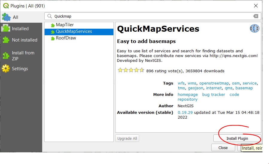
Install the QuickMapServices plugin:
- In the top menu bar, click on Plugins > Manage and Install Plugins.
- In the Plugins dialogue box, search for and install the QuickMapServices plugin.
- To allow us to add additional web layers, on the top menu, click Web > QuickMapServices > Settings. Go to the More Services tab and click Get contributed pack. Close the window.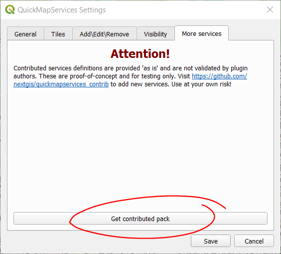
- While the Plugin window is open, also install the qgis2web plugin.
- Once the plugins are installed, close the plugins window.
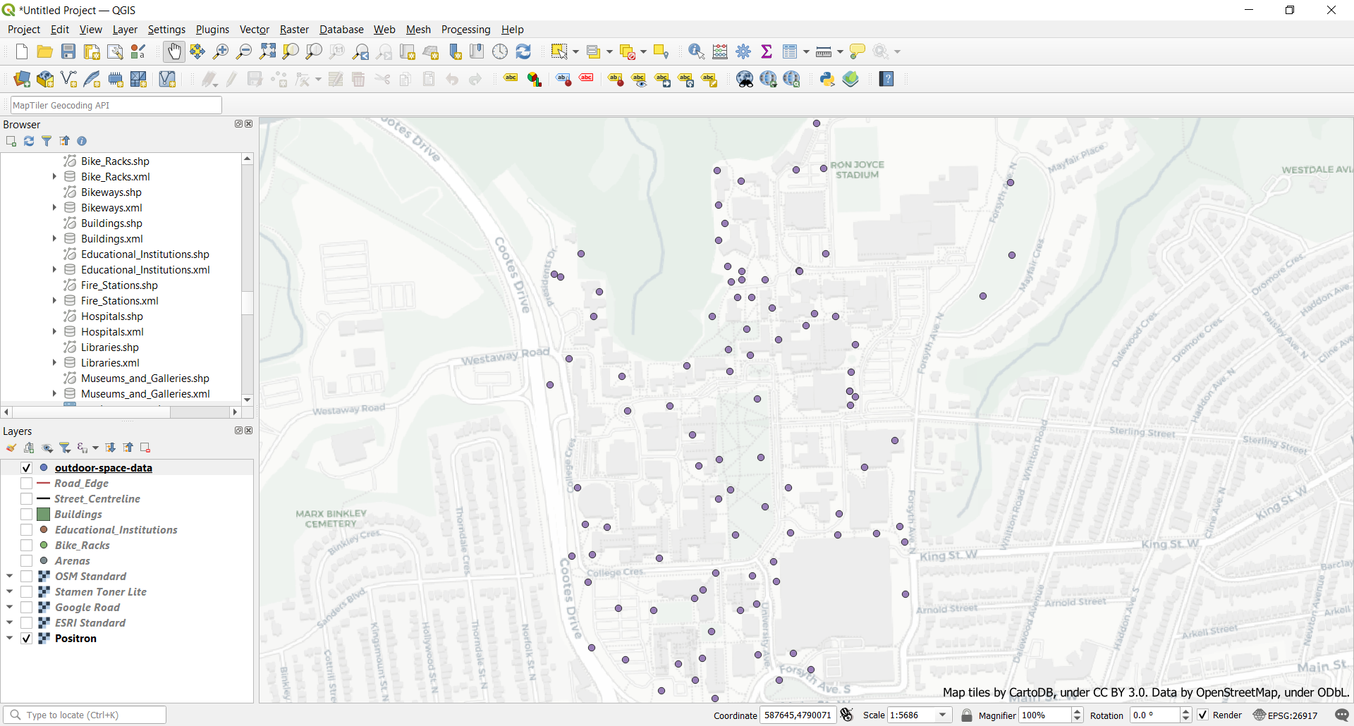
Add a web base map to your data frame:
- In the top menu bar, click on Web > QuickMapServices.
- Explore and add a base map of your liking. Choose a web map for your base map (e.g. check out the OSM and CartoDB maps). Note that some maps (like Stamen) are no longer available and will not display.
- Be sure to right-click and Remove Layer for any layer you don’t want to use.

In the top menu, click on Layer > Add Layer > Add Delimited Text Layer....
Browse to the outdoor-space-data.csv file, select and Open it.
Enter the following information:
- File Format: CSV
- Geometry Definition: X field : Longitude ; Y field : Latitude.
- Geometry CRS: EPSG:4326 - WGS 84
Click Add. When prompted about a transformation, just click OK.
Our survey points should now show on the map in the expected locations (i.e. McMaster University).

Ensure that the outdoor-space-data layer is above your web map in the Layer panel.
Right click the outdoor-space-data layer and select Properties. Click on the Symbology tab
In the top dropdown menu, change to Graduated
In the Value dropdown, select a measure of interest (i.e. Suitability Score)
In the Symbol area, click the current symbol to change it.
- In the symbol dialogue box, click the more options icon beside the Size setting.
- Select Edit. In the Expression box, enter "Num Seats" /10 – this will scale the size of the marker to the number of seats that are available at the location.
- Click OK
Select a Color ramp from the dropdown menu. Be thoughtful with your colour selection: think about what kind of message/sentiment do your selected colours convey. Is it aligned with what you’re communicating in your map?
Click Classify and observe that 5 classes are created. Click Apply to see the changes on the map.
Click OK on the Properties box.
In the Layer Rednering box, edit the transparency of this layer so that the webmap beneath shows a bit.
Click OK to exit the layer properties dialog box.

If you would like to augment your map with other data, add Hamilton Open Data layers and style them appropriately.

Zoom the main data frame to the approximate desired extents for your map.
Click on the New Print Layout button to open the map creation window.
- Give your map a name when the dialog box comes up.
In the map composer, add the critical elements of a map:
- Click the Add new map button and then draw a box to specify your map’s extent on the page. This will draw the contents of your data frame onto the map.
- Use the *Move Item Content button to change the extent and zoom. Click “Update Preview” in the “Main Properties” box to regenerate preview.
WIth the map content selected, go to Item Properties and add a frame (if desired), a grid, or both.
See this video for some examples of how to style the map.

Use Add New Labels button to add any desired labels (Use “Item Properties” tab to control font size, colour, background)
Use the Add North Arrow button to add a North arrow
- With the north arrow selected, scale it to the right size
- Go to > Item Properties to select symbol different than the default.
Use the Add Label button to add a title. Include the creator name and creation date
Use the “Add legend” button to insert a legend, if desired.
- With the legend selected, click the “Item Properties” tab, rename and rearrange the legend items
Use the Add Scale Bar tool to insert a scale bar
- Drag the bar to the desired location and size. Edit other details in the Items Properties box, if desired.
- Set units to Meters, and Label to “m” (if not already done for your)
- Select desired number of segments,

In the map composer, use either the Export as image or Export as PDF buttons to export the map in the desired format to a desired directory.

Save your project and close the map composer window. Keep your project open in the main QGIS interface.

Are you ready for your final challenge? Head to the next lesson to learn how to create and publish a webmap using QGIS and GitHub!